H-Drive Programming

kinganu123 · January 30, 2015, 1:15am

Yes, I didn’t realize that he specified the strafe axis, which would result in the confusion.
And we haven’t been able to test it yet since the mechanical guys are currently assembling the elevator on the robot, so we’re losing a few days on testing and tuning this.
Also, I thought I’d note here that we tweaked the code above, in case anyone else wanted to try our stuff out, because I noticed a slight flaw in getting the y values


centerCurrent = xAxis;
double gaussianInput=angleToGaussianInput(Math.atan2(yAxis, xAxis));
double scaledGaussianOutput=yAxis*gaussianConversion(gaussianInput)
leftCurrent =scaledGaussianOutput+rotate;
rightCurrent=scaledGaussianOutput-rotate;

Ether · January 30, 2015, 9:00am

It’s not just the axis; the gains are quite different from what was described.

I’m a math enthusiast, so don’t take this wrong, but why the complicated function with exponential and inverse trig? Wouldn’t a simple linear interpolated 6x6 LUT do the job… and be far more easily tuned to compensate for actual behavior once you’ve done your testing?

kinganu123 · January 30, 2015, 6:30pm

So we do have a simpler version coded up with some sort of linear adjustment instead of this one (I had some of the other students write that as a backup), but the main reasoning behind this method was to allow y to increase significantly to make up the lost y speed as the driver went at a smaller angle (with respect to the front of the robot).

Ether · February 3, 2015, 5:16pm

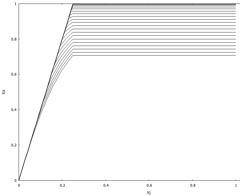
*Instead of using arctangent and exponential functions, why not just multiply the X axis by a factor of 4, clip it at 1, and normalize the resulting X,Y pair?

***

*void adjust(float Xj, float Yj, float *Xa, float *Ya){

	float mag;

	*Ya=Yj;
	
	if (Xj<=-0.25) *Xa=-1; 
	else if (Xj<0.25) *Xa=4.0*Xj;
	else *Xa=1.0;

	// normalize adjusted values:
	mag=sqrt(*Xa**Xa+*Ya**Ya);
	if (mag>1) {*Xa/=mag; *Ya/=mag;}
}**

See attached Excel spreadsheet. The 100 tab shows an overview of adjusted XY pairs (cyan cells) for the entire first quadrant. The 25 tab zooms in for a closer look for small joystick values.

The attached plot shows a family of Xa vs Xj curves for Yj=0 to 1.

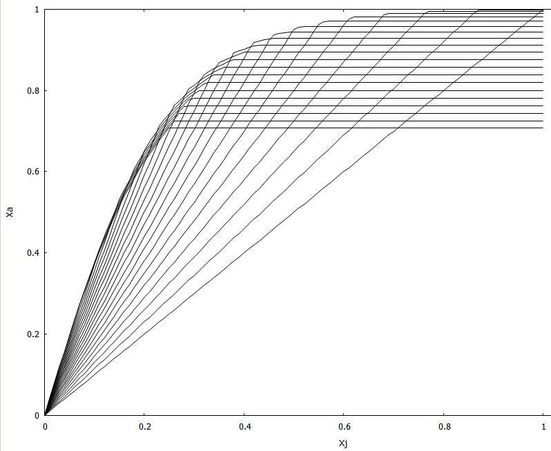
Or you could make the X gain a function of Yj, like so:

***

*void adjust(float Xj, float Yj, float *Xa, float *Ya){

	float mag, gain;

        gain=1+3*Yj;

	*Ya=Yj;
	
        *Xa=gain*Xj;
        if (*Xa>1) *Xa=1;
        else if (*Xa<-1) *Xa=-1;

	// normalize adjusted values:
	mag=sqrt(*Xa**Xa+*Ya**Ya);
	if (mag>1) {*Xa/=mag; *Ya/=mag;}
}**

See attached plots for Xa vs Xj for Yj=0 to 1
and Ya vs Yj for Xj=0 to 1

*

XY.xls (47 KB)

XY.xls (47 KB)